Creating Diagrams with LaTeX

Overview of creating diagrams with LaTeX

TikZ is a powerful and flexible tool for creating high-quality diagrams in LaTeX documents. With TikZ, you can create a wide range of diagrams, including:

Flowcharts: Flowcharts are used to illustrate the flow of a process, such as a software program or a manufacturing process.
Network diagrams: Network diagrams are used to show the relationships between different nodes in a network, such as a computer network or a social network.
Circuit diagrams: Circuit diagrams are used to illustrate electrical circuits, including the connections between different components.
Mind maps: Mind maps are used to illustrate the relationships between different ideas or concepts, such as brainstorming or planning sessions.
Graphs and charts: TikZ can also be used to create a wide range of graphs and charts, including bar charts, line charts, and pie charts.
Venn diagrams: Venn diagrams are used to illustrate the relationships between different sets of data, such as overlapping categories or groups.

Overall, TikZ offers a wide range of possibilities for creating high-quality diagrams in LaTeX documents, making it an invaluable tool for technical writers and academics.

There are several packages and tools available for creating diagrams in LaTeX documents. Some of the most popular ones are:

TikZ: TikZ is a powerful and flexible tool for creating high-quality diagrams in LaTeX documents. It is highly customizable and allows for precise control over every aspect of the diagram.
PGFPlots: PGFPlots is a package for creating 2D and 3D plots in LaTeX documents. It offers a wide range of options for customizing the appearance and layout of the plot.
Circuitikz: Circuitikz is a TikZ-based package for creating high-quality electrical circuit diagrams in LaTeX documents. It offers a wide range of components and symbols for building complex circuits.
Flowchart: Flowchart is a package for creating flowcharts in LaTeX documents. It is easy to use and offers a range of pre-built shapes and symbols for creating complex flowcharts.
Graphviz: Graphviz is a software tool for creating diagrams and graphs. It has a simple syntax for defining nodes and edges, and can generate a wide range of diagram types, including flowcharts, network diagrams, and more.
Dia: Dia is a cross-platform diagramming tool that can be used to create a wide range of diagrams, including flowcharts, network diagrams, and more. It has a simple interface and a wide range of pre-built shapes and symbols.

Overall, there are many tools and packages available for creating diagrams in LaTeX documents, and choosing the right one depends on the specific needs of your project.

The Standalone package is a LaTeX package that allows you to create a separate document for each diagram you create, which can then be compiled into a standalone image file. This is useful when you want to include the diagram in a non-LaTeX document, such as a web page or a presentation.

To use the Standalone package, you simply include the \documentclass{standalone} command at the beginning of your diagram file. You can then add your TikZ or other diagram code as usual. When you compile the document, a standalone PDF file will be generated that contains only the diagram.

However, when you want to include the diagram in a document that does not support PDFs, you need to convert the PDF to a different image format, such as PNG. One way to do this is by using ImageMagick, a free and open-source software tool for manipulating images.

To convert a PDF to a PNG using ImageMagick, you can use the following command in the terminal:

convert -density 300 diagram.pdf -quality 90 diagram.png

This command converts the PDF file “diagram.pdf” to a PNG file “diagram.png” with a density of 300 DPI and a quality of 90%.

Overall, the Standalone package and ImageMagick are powerful tools that can help you create high-quality diagrams for use in a variety of different contexts. By using these tools, you can create diagrams that are both precise and visually appealing, and that can be easily incorporated into a wide range of documents and presentations.

Basic diagrams with TikZ

TikZ is a powerful and flexible package for creating high-quality diagrams in LaTeX documents. It provides a wide range of tools for creating basic diagrams, such as lines, circles, rectangles, and polygons, as well as more complex shapes and structures, such as trees and graphs.

To use TikZ, you start by including the package in your LaTeX document with the command \usepackage{tikz}. You can then add your TikZ code within a tikzpicture environment, like this:

\begin{tikzpicture}
% TikZ code goes here
\end{tikzpicture}

Within the tikzpicture environment, you can create a wide range of shapes and structures using TikZ commands. For example, to create a line, you can use the \draw command, like this:

s\draw (0,0) -- (2,2);

This creates a line that starts at the point (0,0) and ends at the point (2,2). You can customize the appearance of the line using various TikZ options, such as line width, color, and style.

Similarly, you can create other basic shapes using TikZ commands. For example, to create a circle, you can use the \draw command with the circle option, like this:

s\draw (1,1) circle [radius=1];

This creates a circle with a center at the point (1,1) and a radius of 1 unit.

Overall, TikZ is a powerful and flexible tool for creating basic diagrams in LaTeX documents. By using TikZ commands and options, you can create a wide range of shapes and structures that can be customized to meet your specific needs.

TikZ is a powerful and flexible package for creating high-quality diagrams in LaTeX documents. It provides a wide range of tools for creating shapes, lines, arrows, and other structures. In this post, we will introduce the TikZ syntax and commands for creating these elements.

To start using TikZ, you first need to include the package in your LaTeX document with the command \usepackage{tikz}. You can then add your TikZ code within a tikzpicture environment, like this:

\begin{tikzpicture}
% TikZ code goes here
\end{tikzpicture}

Within the tikzpicture environment, you can create a wide range of shapes and structures using TikZ commands. Here are some of the most common ones:

Lines: To create a line, you can use the \draw command, like this:

s\draw (0,0) -- (2,2);

This creates a line that starts at the point (0,0) and ends at the point (2,2).

Shapes: To create a shape, you can use the \draw command with a shape option, like this:

s\draw (1,1) circle [radius=1];

This creates a circle with a center at the point (1,1) and a radius of 1 unit. You can also create other shapes, such as rectangles and polygons, using various TikZ options.

Arrows: To create an arrow, you can use the \draw command with an arrow option, like this:

s\draw [->] (0,0) -- (2,2);

This creates an arrow that starts at the point (0,0) and ends at the point (2,2). You can customize the appearance of the arrow using various TikZ options, such as arrow type and size.

Overall, TikZ is a powerful and flexible tool for creating shapes, lines, arrows, and other structures in LaTeX documents. By using TikZ commands and options, you can create a wide range of diagrams that can be customized to meet your specific needs.

TikZ is a powerful and flexible package for creating high-quality diagrams in LaTeX documents. It can be used to create a wide range of diagrams, including flowcharts, mindmaps, and other basic diagrams. In this post, we will provide an overview of how to use TikZ to create these types of diagrams.

Flowcharts: To create a flowchart, you can use the TikZ library called “shapes.arrows”. This library provides various arrow shapes that can be used to create flowchart elements, such as decision points, input/output boxes, and process boxes. For example, to create a decision point, you can use the diamond shape like this:

\usepackage{tikz}
\usetikzlibrary{shapes.arrows}

\begin{tikzpicture}
\node[diamond, draw, aspect=2] (a) {Decision};
\end{tikzpicture}

This creates a diamond shape with the label “Decision” inside it.

Mindmaps: To create a mindmap, you can use the TikZ library called “mindmap”. This library provides various node shapes and styles that can be used to create a hierarchical structure of nodes. For example, to create a mindmap with three levels of nodes, you can use the mindmap library like this:

\usepackage{tikz}
\usetikzlibrary{mindmap}

\begin{tikzpicture}[mindmap, grow cyclic, every node/.style=concept, concept color=blue!40, level 1/.append style={level distance=5cm, sibling angle=120}, level 2/.append style={level distance=3cm, sibling angle=45}, level 3/.append style={level distance=2cm, sibling angle=60}]
\node{Root Node}
child{node{Level 1 Node 1}
 child{node{Level 2 Node 1}}
 child{node{Level 2 Node 2}}
}
child{node{Level 1 Node 2}
 child{node{Level 2 Node 3}}
 child{node{Level 2 Node 4}}
}
child{node{Level 1 Node 3}
 child{node{Level 2 Node 5}}
 child{node{Level 2 Node 6}}
};
\end{tikzpicture}

This creates a mindmap with a root node and three levels of child nodes.

Other basic diagrams: TikZ can also be used to create other basic diagrams, such as bar charts, pie charts, and Venn diagrams. For example, to create a bar chart, you can use the TikZ library called “pgfplots”. This library provides various plot types and styles that can be used to create bar charts, line charts, and other types of charts. For example, to create a simple bar chart, you can use the pgfplots library like this:

s\usepackage{tikz}
\usepackage{pgfplots}

\begin{tikzpicture}
\begin{axis}[ybar, symbolic x coords={A,B,C,D,E,F}, xtick=data]
\addplot coordinates {(A,3) (B,2) (C,1) (D,4) (E,5) (F,2)};
\end{axis}
\end{tikzpicture}

This creates a bar chart with six bars representing the values 3, 2, 1, 4, 5, and 2 for the categories A, B, C, D, E, and F, respectively.

Overall, TikZ is a powerful and flexible tool

Circuit Diagrams with Circuitikz

Circuitikz is a TikZ-based package for creating circuit diagrams in LaTeX. It provides a comprehensive set of tools for creating electrical and electronic circuits, including resistors, capacitors, inductors, diodes, transistors, and many other components. In this post, we will provide an overview of how to use Circuitikz to create circuit diagrams.

Basic Circuit Elements: Circuitikz provides various basic circuit elements, such as resistors, capacitors, and inductors. These elements can be added to a circuit diagram by simply using the appropriate command. For example, to add a resistor to a circuit diagram, you can use the command:

\usepackage{circuitikz}

\begin{circuitikz}
\draw (0,0) to[R=$R$] (2,0);
\end{circuitikz}

This creates a resistor with a label “R” and connects it to two points at coordinates (0,0) and (2,0) using the “to” command.

Nodes and Labels: Circuitikz also allows you to add nodes and labels to circuit elements. For example, to add a label to a resistor, you can use the “label” command. This command adds a label to the element at a specified position relative to the element. For example:

\begin{circuitikz}
\draw (0,0) to[R=$R$,label=above:$5\,\Omega$] (2,0);
\end{circuitikz}

This creates a resistor with a label “R” and another label “5 $\Omega$” above it.

Advanced Circuit Elements: Circuitikz also provides various advanced circuit elements, such as transistors, op-amps, and logic gates. These elements can be added to a circuit diagram using the appropriate commands. For example, to add a transistor, you can use the command:

s\begin{circuitikz}
\draw (0,0) node[npn](npn){};
\end{circuitikz}

This creates an NPN transistor at coordinates (0,0).

Customization: Circuitikz allows you to customize the appearance of circuit elements by changing various parameters, such as line width, color, and shape. For example, to change the line width of a resistor, you can use the “line width” parameter like this:

\begin{circuitikz}
\draw (0,0) to[R=$R$,line width=2pt] (2,0);
\end{circuitikz}

This creates a resistor with a thicker line.

Overall, Circuitikz is a powerful and flexible tool for creating circuit diagrams in LaTeX. Its comprehensive set of tools and customization options make it an ideal choice for anyone looking to create high-quality circuit diagrams in their LaTeX documents.

 \documentclass[tikz]{standalone}
\usepackage{circuitikz}
\usepackage{siunitx}
\usepackage{amsmath,amssymb}
\begin{document}
\begin{circuitikz}
	\draw (0,2) to[V,l_=$4 \si{\volt}$] (0,0); %% Note _>= instead of >=
	\draw (0,2)to [R,l^=$10 \si{\ohm}$] (2,2);
	\draw (2,2)to [cV,l^=$3V_{ab}$] (4,2);
	\draw (4,0) to  [I,l^=$2\si{\ampere}$](4,2);
	\draw (4,2) to [short,-*] (6,2)
		node[label={[font=\footnotesize]right:$a$}] {};
	\draw (0,0) to [short,-*] (6,0)
		node[label={[font=\footnotesize]right:$b$}] {};
	\draw (6,2) to [open,v_>=$V_{ab}$] (6,0);
\end{circuitikz}
\end{document}

\documentclass[tikz]{standalone} \usepackage{circuitikz} \usepackage{siunitx} \usepackage{amsmath,amssymb} \begin{document} \begin{circuitikz} \draw (0,2) to[V,l_=$4 \si{\volt}$] (0,0); %% Note >= instead of >= \draw (0,2)to [R,l^=$10 \si{\ohm}$] (2,2); \draw (2,2)to [cV,l^=$3V{ab}$] (4,2); \draw (4,0) to I,l^=$2\si{\ampere}$; \draw (4,2) to [short,-] (6,2) node[label={[font=\footnotesize]right:$a$}] {}; \draw (0,0) to [short,-] (6,0) node[label={[font=\footnotesize]right:$b$}] {}; \draw (6,2) to [open,v_>=$V_{ab}$] (6,0); \end{circuitikz} \end{document} This code defines a standalone LaTeX document with a TikZ environment for creating an electrical circuit diagram. It includes the necessary packages for creating circuit diagrams, using SI units, and typesetting mathematical symbols.

The circuit consists of a voltage source with a value of 4 volts connected in series to a resistor with a value of 10 ohms. The voltage at the top of the resistor is connected to a controlled voltage source with a voltage of 3 times the voltage between nodes a and b. The bottom of the controlled voltage source is connected to a current source with a value of 2 amperes. Nodes a and b are connected to the top and bottom of the circuit respectively. An open circuit element with a label of Vab is added to the right of the circuit to represent the voltage between nodes a and b.

Circuitikz ]

 \documentclass[tikz]{standalone}
\usepackage{circuitikz}
\usepackage{siunitx}
\usepackage{amsmath,amssymb}
\begin{document}
\begin{circuitikz}[american voltages]
	% Voltage source
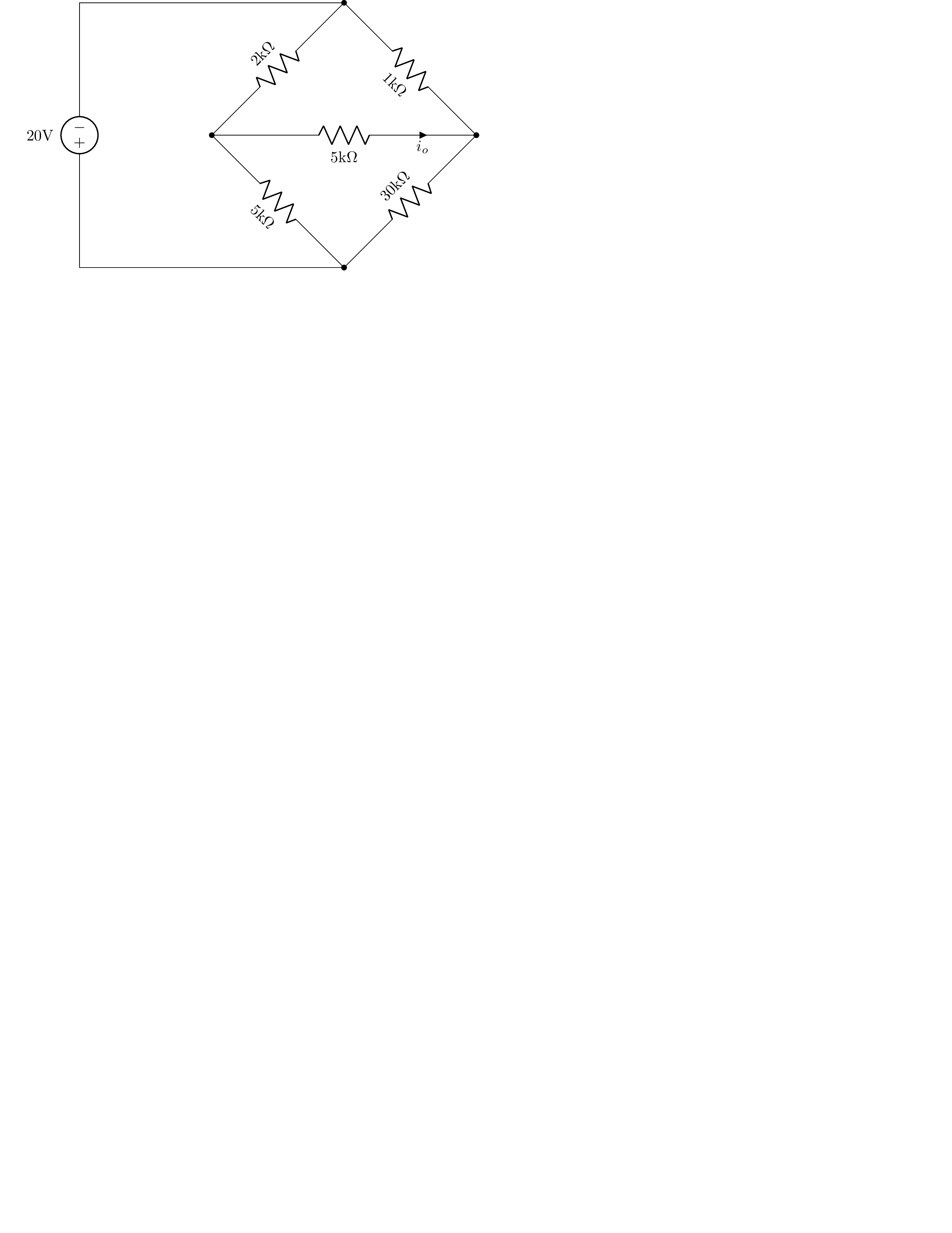
	\draw (0,0) to [V, v>=$20 \si{\volt}$](0, 6) to (6, 6)
	% Left half bridge
	to [R, l_=$2 \si{k\ohm}$, *-*] (3,3) % Top left resistor
	to [R, l_=$5 \si{k\ohm}$, -*] (6,0);  % Bottom left resistor
	% Right half bridge
	\draw (6,6)
	to [R, l_=$1 \si{k\ohm}$, -*] (9, 3) % Top right resistor
	to [R, l_=$30 \si{k\ohm}$, -*] (6,0)  % Bottom left resistor
	% Draw connection to (-) terminal of voltage source
	to (6, 0) to (0,0);
	
	% Draw voltmeter
	\draw (3, 3) to [R, l_=$5 \si{k\ohm}$,i_=$i_o$, -*] (9, 3);
\end{circuitikz}
\end{document}

\documentclass[tikz]{standalone} \usepackage{circuitikz} \usepackage{siunitx} \usepackage{amsmath,amssymb} \begin{document} \begin{circuitikz}[american voltages] % Voltage source \draw (0,0) to [V, v>=$20 \si{\volt}$](0, 6) to (6, 6) % Left half bridge to [R, l_=$2 \si{k\ohm}$, -] (3,3) % Top left resistor to [R, l_=$5 \si{k\ohm}$, -] (6,0); % Bottom left resistor % Right half bridge \draw (6,6) to [R, l_=$1 \si{k\ohm}$, -] (9, 3) % Top right resistor to [R, l_=$30 \si{k\ohm}$, -*] (6,0) % Bottom left resistor % Draw connection to (-) terminal of voltage source to (6, 0) to (0,0);

% Draw voltmeter
\draw (3, 3) to [R, l_=$5 \si{k\ohm}$,i_=$i_o$, -*] (9, 3);

\end{circuitikz} \end{document} This is a LaTeX code that generates a circuit diagram using the circuitikz package. The circuit diagram depicts a voltage source connected to two half bridges, with a voltmeter connected across one of the resistors in the right half bridge. The siunitx and amsmath packages are also included.

The circuit diagram consists of several components and parameters specified using various circuitikz commands. The voltage source is created using the V command, with a voltage of 20 volts and labeled with the v parameter. The resistors are created using the R command, with their values specified using the l parameter, and their orientation specified using the - and * parameters. The voltmeter is created using another R command, and is labeled with the i parameter. The american voltages option is used to display voltages in the diagram in the American style.

Circuitikz ]

 \documentclass[tikz]{standalone}
\usepackage{circuitikz}
\usepackage{siunitx}
\usepackage{amsmath,amssymb}
\begin{document}
\begin{circuitikz}
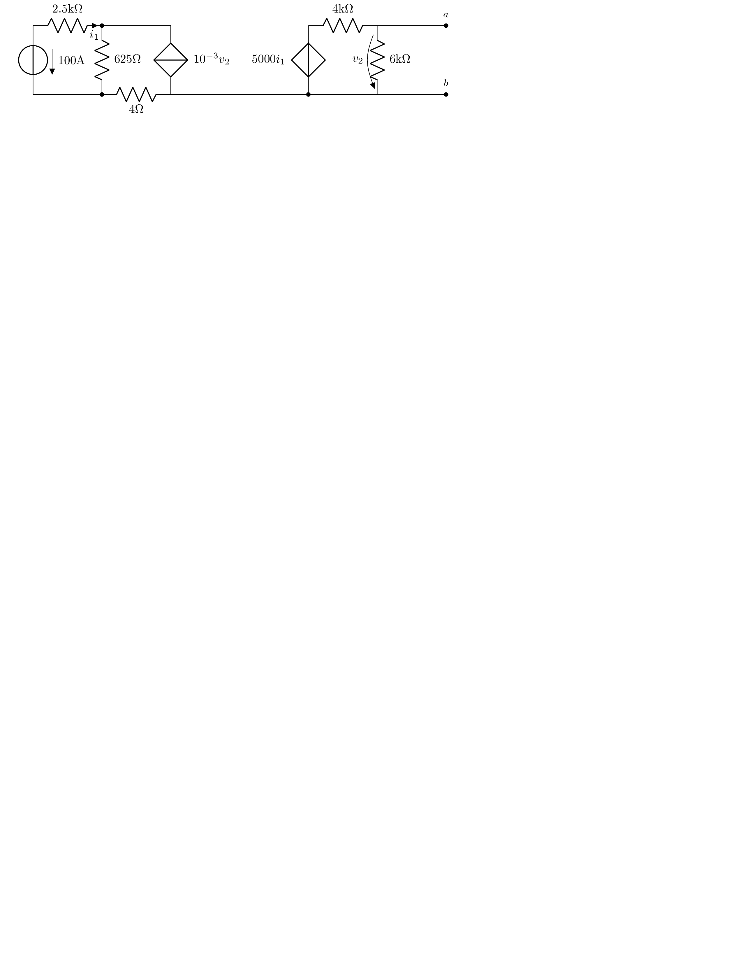
	\draw (0,2) to[V,v>=$100\si{\ampere}$] (0,0); %% Note _>= instead of >=
	\draw (0,2) to [R,l^=$2.5 \si{k\ohm}$,i_>=$i_1$,-*] (2,2)
	to [R=$625\si{\ohm}$,-*](2,0);
	\draw (2,2) to [short] (4,2);
	\draw (4,0)to [cI,l_=$10^{-3}v_2$] (4,2);
	\draw (4,0)
	to [R,l^=$4\si{\ohm}$] (2,0);
	\draw (0,0) to [short,-*] (2,0);
	
	\draw (4,0) to [short,-*] (8,0);
	\draw (8,2)to [cV,l_=$5000i_1$](8,0)
	to [short] (10,0);
	\draw (8,2)
	to [R,l^=$4\si{k \ohm}$] (10,2)
	to [R,l^=$6\si{k \ohm}$,v_>=$v_2$] (10,0)
	to [short, -*] (12,0)
	node[label={[font=\footnotesize]above:$b$}] {}
	;
	
	\draw (10,2) to [short, -*] (12,2)
	node[label={[font=\footnotesize]above:$a$}] {}
	;
\end{circuitikz}
\end{document}

\draw (4,0) to [short,-*] (8,0);
\draw (8,2)to [cV,l_=$5000i_1$](8,0)
to [short] (10,0);
\draw (8,2)
to [R,l^=$4\si{k \ohm}$] (10,2)
to [R,l^=$6\si{k \ohm}$,v_>=$v_2$] (10,0)
to [short, -*] (12,0)
node[label={[font=\footnotesize]above:$b$}] {}
;

\draw (10,2) to [short, -*] (12,2)
node[label={[font=\footnotesize]above:$a$}] {}
;

\end{circuitikz} \end{document} This is a LaTeX document that uses the standalone document class and several packages including circuitikz, siunitx, and amsmath. The circuitikz package provides the tools to draw electronic circuits, while siunitx provides support for typesetting units and amsmath provides additional math symbols.

The code uses the circuitikz environment to draw a circuit diagram with several components. The circuit consists of a voltage source (V), resistors (R), a current-controlled current source (cI), and a current-controlled voltage source (cV). The components are connected using to commands, and labels are added to indicate the values of resistors and sources, as well as the direction and name of currents and voltages. Labels are also added to nodes in the circuit for later reference.

TheveinEquivalent ]

Control Systems with Tikz

TikZ is a powerful package that can be used to create various types of diagrams in LaTeX, including block diagrams. Block diagrams are a type of diagram that show the flow of a system or process through a series of interconnected blocks or nodes.

To create a block diagram in TikZ, you can follow these steps:

Load the TikZ package by adding the following line to your LaTeX document:

\usepackage{tikz}

Begin a TikZ picture environment by adding the following code:

\begin{tikzpicture}
% TikZ code goes here
\end{tikzpicture}

Define the blocks or nodes of the block diagram using the “node” command. For example, to create a rectangular block, you can use the following code:

s\node [rectangle, draw] (block1) {Block 1};

This creates a rectangular block with the label “Block 1” and assigns it the name “block1”.

Connect the blocks using the “draw” command. For example, to connect two blocks with an arrow, you can use the following code:

s\draw [->] (block1) -- (block2);

This creates an arrow that connects the block named “block1” to the block named “block2”.

Repeat steps 3-4 to add additional blocks and connections to the diagram.

Here is an example of a simple block diagram created using TikZ:

s\begin{tikzpicture}
\node [rectangle, draw] (block1) {Block 1};
\node [rectangle, draw, right of=block1, node distance=3cm] (block2) {Block 2};
\draw [->] (block1) -- (block2);
\end{tikzpicture}

This creates a block diagram with two rectangular blocks labeled “Block 1” and “Block 2”, respectively, and an arrow that connects them.

Overall, TikZ provides a flexible and powerful toolset for creating block diagrams in LaTeX. By using the “node” and “draw” commands, you can easily create and connect blocks to represent the flow of a system or process. With a little practice, you can create complex block diagrams with ease using TikZ.

 \documentclass{standalone}

\usepackage{blox}
\usepackage{tikz}
\usetikzlibrary{positioning}

\begin{document}
\begin{tikzpicture}
%\bXLineStyle{red, dotted}
\bXLineStyle{very thick}
\bXInput{A}
\bXComp{B}{A}
\bXLink[R]{A}{B}
\bXCompa{C}{B}
\bXLink{B}{C}
\bXSumb{D}{C}
\bXLink{C}{D}
\bXBloc[2]{E}{$G_1$}{D}
\bXLink{D}{E}
\bXBloc[2]{F}{$G_2$}{E}
\bXLink{E}{F}

\bXBranchx[5]{F}{FX1}

\bXBranchy[5]{FX1}{FDown1}
\draw[-,very thick] (F) -- (FX1.center);
\draw[-,very thick] (FX1.center) -- (FDown1.center);
\bXBranchx[-5.5]{FDown1}{FRight1}
\draw[->,very thick] (FDown1.center) -- (FRight1.center);
\bXBloc[-3.5]{H1}{$H_1$}{FRight1}
\bXBranchy[5]{D}{DDown1}
\draw[->,very thick] (DDown1.center) -- (D);
\draw[-,very thick] (H1) -- (DDown1.center);

\bXBloc[2]{G}{$G_3$}{FX1}
%\draw[-,very thick]  (F)  -- (FX1);
\draw[->,very thick] (F) -- (G);

\bXBranchx[3]{G}{GX1}
\bXBranchx[3]{GX1}{GX2}
\draw[-,very thick] (G) -- (GX2);
\bXBranchx[3]{GX2}{GX3}
\bXBranchy[-5]{GX2}{GUp1}

\bXBranchx[1.5]{GX2}{GX4}
\bXBranchy[7.5]{GX4}{GDown1}
%\draw[-,very thick] (G) -- (GX1.center);
%\draw[-,very thick] (G) -- (GX1.center);
%\draw[-,very thick] (GX1.center) -- (GUp1.center);
%\bXLinkxy{GX1}{GUp1}
\draw[-,very thick] (GX1.center) -- (GX2.center);
\draw[-,very thick] (GX2.center) -- (GUp1.center);
\draw[->,very thick] (GX2.center) -- (GX3.center);
\node[right = 0.05cm of GX3] (end) {$C$};

\draw[-,very thick] (GX4.center) -- (GDown1.center);

\bXBranchy[7.5]{B}{BDown1}
\bXLink{BDown1.center}{B}
\draw[-,very thick] (GDown1.center) -- (BDown1.center);


%% Top Part

\bXBranchx[-20]{GUp1}{GLUp1}
\bXBloc[-0]{BlockHG}{$\frac{H_2}{G_1}$}{GLUp1}
\draw[->,very thick] (GUp1.center) -- (BlockHG);
\bXLinkxy{BlockHG}{C}
\end{tikzpicture}
\end{document}

\documentclass{standalone}

\usepackage{blox} \usepackage{tikz} \usetikzlibrary{positioning}

\begin{document} \begin{tikzpicture} %\bXLineStyle{red, dotted} \bXLineStyle{very thick} \bXInput{A} \bXComp{B}{A} \bXLink[R]{A}{B} \bXCompa{C}{B} \bXLink{B}{C} \bXSumb{D}{C} \bXLink{C}{D} \bXBloc[2]{E}{$G_1$}{D} \bXLink{D}{E} \bXBloc[2]{F}{$G_2$}{E} \bXLink{E}{F}

\bXBranchx[5]{F}{FX1}

\bXBranchy[5]{FX1}{FDown1} \draw[-,very thick] (F) — (FX1.center); \draw[-,very thick] (FX1.center) — (FDown1.center); \bXBranchx[-5.5]{FDown1}{FRight1} \draw[->,very thick] (FDown1.center) — (FRight1.center); \bXBloc[-3.5]{H1}{$H_1$}{FRight1} \bXBranchy[5]{D}{DDown1} \draw[->,very thick] (DDown1.center) — (D); \draw[-,very thick] (H1) — (DDown1.center);

\bXBloc[2]{G}{$G_3$}{FX1} %\draw[-,very thick] (F) — (FX1); \draw[->,very thick] (F) — (G);

\bXBranchx[3]{G}{GX1} \bXBranchx[3]{GX1}{GX2} \draw[-,very thick] (G) — (GX2); \bXBranchx[3]{GX2}{GX3} \bXBranchy[-5]{GX2}{GUp1}

\bXBranchx[1.5]{GX2}{GX4} \bXBranchy[7.5]{GX4}{GDown1} %\draw[-,very thick] (G) — (GX1.center); %\draw[-,very thick] (G) — (GX1.center); %\draw[-,very thick] (GX1.center) — (GUp1.center); %\bXLinkxy{GX1}{GUp1} \draw[-,very thick] (GX1.center) — (GX2.center); \draw[-,very thick] (GX2.center) — (GUp1.center); \draw[->,very thick] (GX2.center) — (GX3.center); \node[right = 0.05cm of GX3] (end) {$C$};

\draw[-,very thick] (GX4.center) — (GDown1.center);

\bXBranchy[7.5]{B}{BDown1} \bXLink{BDown1.center}{B} \draw[-,very thick] (GDown1.center) — (BDown1.center);

%% Top Part

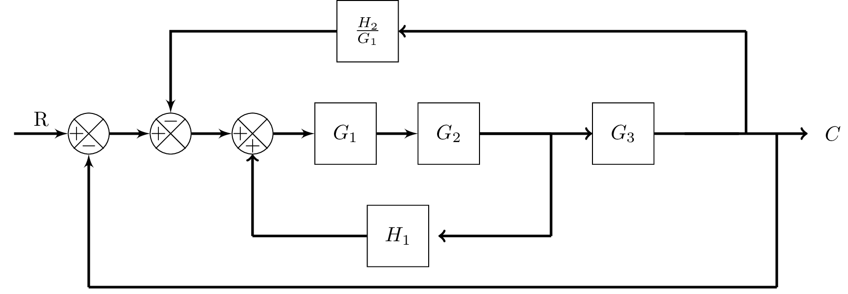
\bXBranchx[-20]{GUp1}{GLUp1} \bXBloc[-0]{BlockHG}{$\frac{H_2}{G_1}$}{GLUp1} \draw[->,very thick] (GUp1.center) — (BlockHG); \bXLinkxy{BlockHG}{C} \end{tikzpicture} \end{document} The code above is a LaTeX document that creates a block diagram using the blox and tikz packages. The block diagram consists of several blocks and arrows that represent a system of interconnected components. The code defines the layout and styling of the blocks and arrows using various blox commands and tikz drawing commands. The document begins with the \documentclass command, which specifies the document class as standalone. The necessary packages are then loaded using the \usepackage command. Finally, the tikzpicture environment is used to create the block diagram using the defined blox and tikz commands.

Block ]

 \documentclass{standalone}
\usepackage{amsmath}  % For math
\usepackage{amssymb}  % For more math

\usepackage{blox}
\usepackage{tikz}
\begin{document}
\begin{tikzpicture}
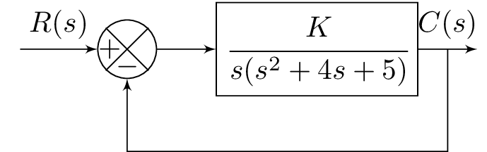
\bXInput{A}
\bXComp{B}{A}
\bXLink[$R(s)$]{A}{B}
\bXBloc[2]{C}{$\cfrac{K}{s(s^2+4s+5)}$}{B}
%\bXLink[$V_1$]{B}{C}
\bXLink{B}{C}
\bXOutput{E}{C}
\bXLink[$C(s)$]{C}{E}
\bXReturn{C-E}{B}{}
\end{tikzpicture}

\end{document}

\documentclass{standalone} \usepackage{amsmath} % For math \usepackage{amssymb} % For more math

\usepackage{blox} \usepackage{tikz} \begin{document} \begin{tikzpicture} \bXInput{A} \bXComp{B}{A} \bXLink[$R(s)$]{A}{B} \bXBloc[2]{C}{$\cfrac{K}{s(s^2+4s+5)}$}{B} %\bXLink[$V_1$]{B}{C} \bXLink{B}{C} \bXOutput{E}{C} \bXLink[$C(s)$]{C}{E} \bXReturn{C-E}{B}{} \end{tikzpicture}

\end{document} The code above is a LaTeX document that defines a TikZ picture environment to create a block diagram. It uses the “blox” package and “tikz” package to draw the blocks and arrows in the diagram. The block diagram represents a feedback control system with an input signal $R(s)$, a controller block with transfer function $\frac{K}{s(s^2+4s+5)}$, and an output signal $C(s)$. The blocks are labeled with letters A, B, C, and E, and arrows are labeled with text to indicate the input and output signals. The “amsmath” and “amssymb” packages are also loaded to allow for mathematical notation in the diagram.

Block ] TikZ is a great tool for creating control systems diagrams in LaTeX for a variety of reasons:

High quality output: TikZ produces high-quality output that can be easily customized to meet specific requirements. This is especially important when creating diagrams for technical documents, where precision and clarity are key.
Flexibility: TikZ provides a wide range of options for creating diagrams. It is possible to create everything from simple block diagrams to complex control systems diagrams with multiple feedback loops.
Integration with LaTeX: TikZ integrates seamlessly with LaTeX, which means that it is easy to include diagrams in technical documents without having to switch to a separate application.
Scalability: TikZ allows you to create scalable diagrams that can be easily resized without losing quality. This is particularly useful when diagrams need to be included in presentations or printed documents of different sizes.
Reusability: TikZ allows you to create templates for frequently used diagrams, which can save time and effort in the long run.
Consistency: TikZ provides a consistent look and feel for all diagrams created using the package. This makes it easy to maintain a consistent style throughout a technical document.

Overall, TikZ is a powerful and flexible tool for creating control systems diagrams in LaTeX. Its integration with LaTeX, high-quality output, and scalability make it an ideal choice for technical documents that require precise and professional-looking diagrams.

Diagrams with PGFPlots

PGFPlots is a powerful package for creating advanced diagrams such as graphs and plots in LaTeX. It is built on top of TikZ and provides a comprehensive set of tools for visualizing data in a variety of formats. Here is an overview of some of the key features of PGFPlots:

Plotting functions: PGFPlots provides a wide range of functions for creating different types of plots, including scatter plots, line plots, bar charts, and more. It also allows you to plot mathematical functions directly, which is particularly useful for visualizing mathematical concepts.
Customization: PGFPlots provides a wide range of customization options for all aspects of the plot, including the axis labels, legend, colors, and styles. This allows you to create plots that are tailored to your specific needs.
Multiple plots: PGFPlots allows you to create multiple plots on the same axis, which is useful for comparing data sets or visualizing different aspects of a single data set.
3D plots: PGFPlots provides tools for creating 3D plots, including surface plots and contour plots. This is particularly useful for visualizing data sets that have three or more dimensions.
Data file support: PGFPlots allows you to import data from external files, including CSV and TSV files. This makes it easy to create plots from data sets stored in other applications or generated by other scripts.
Publication quality output: PGFPlots produces high-quality output that is suitable for use in publications or presentations. It provides tools for adjusting the resolution and size of the output, as well as tools for exporting the output to various file formats, including PDF, PNG, and EPS.

Overall, PGFPlots is a powerful and flexible package for creating advanced diagrams such as graphs and plots in LaTeX. Its wide range of features and customization options make it an ideal choice for visualizing data in a variety of formats, from simple scatter plots to complex 3D visualizations.

PGFPlots is built on top of TikZ, so it uses a similar syntax for creating graphs and plots. Here is an overview of some of the key commands and syntax for creating various types of graphs and plots in PGFPlots:

Axis environment: The axis environment is the main environment for creating plots in PGFPlots. It defines the plot area and provides options for configuring the axis labels, legends, and styles.
Plotting functions: PGFPlots provides a wide range of functions for creating different types of plots. For example, to create a scatter plot, you can use the \addplot command with the scatter option. To create a line plot, you can use the \addplot command with the smooth option.
Axis labels: To add labels to the x-axis and y-axis, you can use the xlabel and ylabel options, respectively. You can also use the title option to add a title to the plot.
Legends: To add a legend to the plot, you can use the legend option. You can specify the legend entries using the \addlegendentry command.
Styles: PGFPlots provides a wide range of styles for customizing the appearance of the plot. For example, you can use the color option to change the color of the plot, the mark option to change the shape of the plot markers, and the line width option to change the thickness of the plot lines.
Multiple plots: PGFPlots allows you to create multiple plots on the same axis using the \addplot command with different data sets or functions. You can use the legend option to specify the legend entries for each plot.
3D plots: To create 3D plots in PGFPlots, you can use the surf option with the \addplot3 command. You can also add contour lines using the contour option.

Overall, PGFPlots provides a comprehensive set of tools for creating a wide range of graphs and plots in LaTeX. Its syntax is similar to TikZ, so it should be familiar to users who are already familiar with TikZ. With its customization options and flexibility, PGFPlots is an ideal choice for visualizing data in a variety of formats.

PGFPlots is a powerful tool for creating a wide range of advanced diagrams, including bar graphs, line graphs, scatter plots, and more. Here’s a brief overview of how to create some of these types of plots using PGFPlots:

Bar graphs: To create a bar graph, you can use the ybar option with the \addplot command. You can also use the bar width option to adjust the width of the bars. You can add multiple bar plots to the same axis using the \addplot command with different data sets.
Line graphs: To create a line graph, you can use the smooth option with the \addplot command. You can also customize the appearance of the lines using options such as color, line width, and mark.
Scatter plots: To create a scatter plot, you can use the scatter option with the \addplot command. You can customize the appearance of the markers using options such as mark, mark size, and color. You can also add a trend line to the scatter plot using the smooth option.
Heatmaps: To create a heatmap, you can use the matrix plot option with the \addplot command. You can specify the data using a matrix, and you can customize the appearance of the heatmap using options such as colormap, point meta min, and point meta max.
3D plots: To create a 3D plot, you can use the surf option with the \addplot3 command. You can also add contour lines using the contour option. You can customize the appearance of the plot using options such as view, zmin, and zmax.
Polar plots: To create a polar plot, you can use the polaraxis environment. You can add multiple plots to the same polar axis using the \addplot command with different data sets. You can customize the appearance of the plot using options such as domain, color, and line width.

These are just a few examples of the types of advanced diagrams that can be created using PGFPlots. With its comprehensive set of tools for customization and its flexible syntax, PGFPlots is a versatile tool for visualizing data in LaTeX.

Git is a powerful version control system that can be used to track changes to files, including LaTeX documents, and collaborate with other authors. Here’s an overview of how to use Git for tracking changes and collaborating on LaTeX documents:

Install Git: The first step is to install Git on your computer. Git is a command-line tool, so you’ll need to be comfortable using the terminal or command prompt. You can download Git from the official website: https://git-scm.com/downloads
Create a Git repository: Once you have Git installed, you can create a new Git repository for your LaTeX project. Navigate to the directory where your LaTeX files are stored and run the command git init to create a new repository. This will create a hidden .git directory in your project directory that Git will use to track changes.
Add files to the repository: To start tracking changes to your LaTeX files, you need to add them to the Git repository. You can do this using the git add command. For example, to add all the files in your project directory, run git add ..
Make commits: Once your files are added to the repository, you can start making commits. A commit is a snapshot of your project at a particular point in time. To make a commit, use the command git commit -m "commit message". The commit message should briefly describe the changes you’ve made.
Collaborate with other authors: If you’re working with other authors, you can use Git to collaborate on the same LaTeX documents. To do this, you’ll need to set up a remote repository, such as on GitHub or GitLab, and give your collaborators access. You can then push your commits to the remote repository using the command git push. Your collaborators can pull your changes using the command git pull.
Manage branches: Git also allows you to create and manage branches, which are separate copies of your project that can be worked on independently. This is useful for experimenting with new features or fixing bugs without affecting the main project. You can create a new branch using the command git branch branch-name and switch to it using git checkout branch-name.

These are just a few examples of how to use Git for tracking changes and collaborating on LaTeX documents. Git can take some time to learn, but once you’re comfortable with it, it can be a powerful tool for managing complex projects and working with other authors.

Best practices for creating diagrams with LaTeX

Here are some tips for efficient diagram creation with TikZ and PGFPlots:

Plan your diagram before starting: Take some time to sketch out the diagram you want to create, and think about the elements you’ll need (shapes, lines, labels, etc.). This will help you avoid making mistakes and save time later on.
Use templates and examples: There are many resources available online for TikZ and PGFPlots, including templates and examples. These can be a great starting point for your own diagrams, and can save you time and effort.
Use libraries: TikZ and PGFPlots both have many libraries of predefined shapes, styles, and functions. These can help you create complex diagrams quickly and easily.
Keep it simple: It can be tempting to add lots of bells and whistles to your diagrams, but simpler diagrams are often clearer and easier to understand. Try to use only the elements you need, and avoid adding unnecessary complexity.
Use macros: If you find yourself repeating the same code over and over again, consider creating a macro. Macros can be defined using \newcommand in LaTeX, and can save you time and reduce errors.
Test your code: As with any programming, it’s important to test your code as you go along. Compile your document frequently and check for errors or unexpected behavior.
Document your code: Finally, make sure to document your code. Use comments to explain what each section of code does, and provide context for the reader. This will make it easier for you and others to understand your code later on.

By following these tips, you can create efficient and effective diagrams with TikZ and PGFPlots.

Here are some common errors that you may encounter when using TikZ and PGFPlots, and some tips for troubleshooting them:

“Package TikZ Error: …”: This error usually indicates that there is a problem with your TikZ code. Check the line number indicated in the error message, and look for syntax errors or missing elements (such as closing brackets).
“Package PGFPlots Error: …”: This error is similar to the TikZ error above, but indicates a problem with your PGFPlots code. Check the line number indicated in the error message, and look for syntax errors or missing elements.
“Dimension too large”: This error occurs when you try to draw a shape or line that is too large for LaTeX to handle. You can try using the fpu library in TikZ, which provides floating-point arithmetic and can handle larger values.
“File not found”: This error can occur when you try to include a file (such as an image or data file) that LaTeX cannot find. Double-check the file path and name, and make sure the file is in the correct location.
“Undefined control sequence”: This error occurs when you use a command that LaTeX does not recognize. Check the spelling of the command and make sure it is spelled correctly.
“Misplaced alignment tab character &”: This error occurs when you use the & character in the wrong context (usually in a table or matrix). Make sure you are using the & character within the correct environment.
“Package xcolor Error: Undefined color”: This error occurs when you use a color that is not defined in the xcolor package. Check the spelling of the color and make sure it is spelled correctly.

To troubleshoot these errors, try the following steps:

Check the error message for clues about what went wrong.
Check the line number indicated in the error message.
Look for syntax errors or missing elements in your code.
Consult the TikZ or PGFPlots documentation for more information about specific commands or options.
Try commenting out parts of your code to isolate the problem.
Ask for help on forums or from colleagues who have experience with TikZ and PGFPlots.

By following these troubleshooting steps and staying familiar with the common errors that can occur, you can save time and frustration when creating diagrams with TikZ and PGFPlots.

Here are some tips for maintaining consistency in diagram formatting and layout:

Define a consistent style: Decide on a consistent style for your diagrams, including font, colors, line styles, and arrowheads. Use this style consistently across all of your diagrams to ensure a cohesive and professional look.
Use templates: Create a template for each type of diagram you need to create, including all of the necessary formatting and layout elements. This will help ensure that all of your diagrams have a consistent look and feel.
Use layers: Use layers to organize your diagram elements and make it easier to modify them. For example, you could use separate layers for text, shapes, and lines, and keep the layers consistent across all of your diagrams.
Label elements consistently: Use consistent labeling for all of your diagram elements, including text, shapes, and lines. For example, use the same label for a certain type of line or arrowhead across all of your diagrams.
Use a grid: Use a grid to ensure that your diagram elements are aligned properly. This will help give your diagrams a consistent look and make them easier to read.
Keep it simple: Avoid cluttering your diagrams with too many elements. Stick to the essential information, and use a clear and simple layout to make your diagrams easy to read.
Get feedback: Ask for feedback from colleagues or others who are familiar with your diagrams. They can help identify any inconsistencies or areas where you could improve your layout and formatting.

By following these tips, you can maintain consistency in your diagram formatting and layout, making your diagrams easier to read and giving them a professional look.

 % Dupplicated from https://code.visualstudio.com/docs/remote/containers
\documentclass[11pt]{standalone}
\usepackage[T1]{fontenc}
\usepackage{tikz}
\usetikzlibrary{calc,positioning,shapes.geometric}
\begin{document}
  \begin{tikzpicture}[
    >=stealth,
    node distance=1cm,
    orange/.style={
      minimum width = 11em,
      fill=orange!50,
      draw=red!40,
      text width = 0.35\textwidth,
      text centered,
    },
    database/.style={
      cylinder,
      cylinder uses custom fill,
      cylinder body fill=green!60!black!50,
      cylinder end fill=green!10,
      shape border rotate=90,
      aspect=0.25,
      draw
    }
  ]
   
    \node[rounded corners, %fill=black,
    text depth = 5em,
    draw=blue!80,
    % double distance =1pt,    %% here
    %font=\Large, 
    minimum height= 20em,
    minimum width= 20em,
    label={[anchor=north, color=blue!90, inner sep=0pt, xshift=3em, yshift=-1em] north west:{Local OS}}]  (dw){};
    
        \node[rounded corners, %fill=black,
    text depth = 5em,
    draw=blue!80,
    % double distance =1pt,    %% here
    %font=\Large, 
    minimum height= 20em,
    minimum width= 30em,
    label={[anchor=north, color=blue!90, inner sep=0pt, xshift=3em, yshift=-1em] north west:{Container}},
    right = of dw]  (container){};
    \node[ %fill=black,
    draw=blue!90,
    text centered,
    text width = 0.20\textwidth,
    fill=blue!50,
    minimum height= 7em,
    minimum width= 15em,
    label={[anchor=north, inner sep=0pt, yshift=-0.2em] north:{\Large \textcolor{white}{VS Code}}}] at ([yshift=2em] dw.center) (code){};
    \node[orange] at ([yshift=-1.25em] code.center) (t1) {Theme/UI Extension} ;
    \node[orange] at ([yshift= 0.75em] code.center) (t2) {Theme/UI Extension};
  
    \node[ %fill=black,
    draw=blue!90,
    text centered,
    text width = 0.20\textwidth,
    fill=blue!50,
    minimum height= 7em,
    minimum width= 15em,
    label={[anchor=north, inner sep=0pt, yshift=-0.2em] north:{\Large \textcolor{white}{VS Code Server}}}] at ([xshift=10em, yshift=2em] container.west) (codeserver){};
    \node[orange] at ([yshift=-1.25em] codeserver.center) (we1) {WorkSpace Extension} ;
    \node[orange] at ([yshift= 0.75em] codeserver.center) (we2) {WorkSpace Extension};
    
    % Data Sources
      
    % Source Code
    \node[database] (db1) at ([yshift=-5em] code.south) (scOS) {Source Code};
    \node[database, opacity=0.6] (db1) at ([yshift=-5em] codeserver.south) (scContainer) {Source Code};
    % Container Stuff

    % Container widgets
        % Configuration Files and Plugin box
    \node[
    draw=black!10,
    text centered,
    fill=green!30,
    minimum width= 10em] at ([xshift=7em, yshift=-3em] codeserver.north east) (tp){Terminal Processes};
        \node[
    draw=black!10,
    text centered,
    fill=green!30,
    minimum width= 10em] at ([xshift=7em, yshift=-5em] codeserver.north east) (ra){Running Application};
            \node[
    draw=black!10,
    text centered,
    fill=green!30,
    minimum width= 10em] at ([xshift=7em, yshift=-7em] codeserver.north east) (debug){Debugger};
    
     \node[database] (db1) at ([yshift=2em, xshift=7em] codeserver.north east) (fs) {File System};
     
     % Connect and labels
    
    % Arrows 
    \draw[->, very thick, draw=blue!40] (code.east) -> (codeserver.west);
    % Labels
    \node[rounded corners, %fill=black,
    draw=none,
    minimum height= 2em,
    fill = white,
    % double distance =1pt,    %% here
    %font=\Large, 
    text width = 0.11\textwidth,
    text centered,
    minimum width=1.5em,
    xshift=3.75em] at (code.east) (dw1){Exposed port};
    
    \draw[->, very thick, draw=blue!40] (scOS.east) -> (scContainer.west);
    \node[rounded corners, %fill=black,
    draw=none,
    minimum height= 2em,
    fill = white,
    % double distance =1pt,    %% here
    %font=\Large, 
    text width = 0.11\textwidth,
    text centered,
    minimum width=1.5em,
    xshift=8.25em] at (scOS.east) (dw1){Volume Mount};
    \draw[->, very thick, draw=blue!40] (codeserver) -> (fs.west);
    \draw[->, very thick, draw=blue!40] (codeserver) -> (tp);
    \draw[->, very thick, draw=blue!40] (codeserver) -> (ra.west);
    \draw[->, very thick, draw=blue!40] (codeserver) -> (debug.west);
    \end{tikzpicture}
\end{document}

% Dupplicated from https://code.visualstudio.com/docs/remote/containers \documentclass[11pt]{standalone} \usepackage[T1]{fontenc} \usepackage{tikz} \usetikzlibrary{calc,positioning,shapes.geometric} \begin{document} \begin{tikzpicture}[ >=stealth, node distance=1cm, orange/.style={ minimum width = 11em, fill=orange!50, draw=red!40, text width = 0.35\textwidth, text centered, }, database/.style={ cylinder, cylinder uses custom fill, cylinder body fill=green!60!black!50, cylinder end fill=green!10, shape border rotate=90, aspect=0.25, draw } ]

\node[rounded corners, %fill=black,
text depth = 5em,
draw=blue!80,
% double distance =1pt,    %% here
%font=\Large, 
minimum height= 20em,
minimum width= 20em,
label={[anchor=north, color=blue!90, inner sep=0pt, xshift=3em, yshift=-1em] north west:{Local OS}}]  (dw){};

    \node[rounded corners, %fill=black,
text depth = 5em,
draw=blue!80,
% double distance =1pt,    %% here
%font=\Large, 
minimum height= 20em,
minimum width= 30em,
label={[anchor=north, color=blue!90, inner sep=0pt, xshift=3em, yshift=-1em] north west:{Container}},
right = of dw]  (container){};
\node[ %fill=black,
draw=blue!90,
text centered,
text width = 0.20\textwidth,
fill=blue!50,
minimum height= 7em,
minimum width= 15em,
label={[anchor=north, inner sep=0pt, yshift=-0.2em] north:{\Large \textcolor{white}{VS Code}}}] at ([yshift=2em] dw.center) (code){};
\node[orange] at ([yshift=-1.25em] code.center) (t1) {Theme/UI Extension} ;
\node[orange] at ([yshift= 0.75em] code.center) (t2) {Theme/UI Extension};

\node[ %fill=black,
draw=blue!90,
text centered,
text width = 0.20\textwidth,
fill=blue!50,
minimum height= 7em,
minimum width= 15em,
label={[anchor=north, inner sep=0pt, yshift=-0.2em] north:{\Large \textcolor{white}{VS Code Server}}}] at ([xshift=10em, yshift=2em] container.west) (codeserver){};
\node[orange] at ([yshift=-1.25em] codeserver.center) (we1) {WorkSpace Extension} ;
\node[orange] at ([yshift= 0.75em] codeserver.center) (we2) {WorkSpace Extension};

% Data Sources
  
% Source Code
\node[database] (db1) at ([yshift=-5em] code.south) (scOS) {Source Code};
\node[database, opacity=0.6] (db1) at ([yshift=-5em] codeserver.south) (scContainer) {Source Code};
% Container Stuff

% Container widgets
    % Configuration Files and Plugin box
\node[
draw=black!10,
text centered,
fill=green!30,
minimum width= 10em] at ([xshift=7em, yshift=-3em] codeserver.north east) (tp){Terminal Processes};
    \node[
draw=black!10,
text centered,
fill=green!30,
minimum width= 10em] at ([xshift=7em, yshift=-5em] codeserver.north east) (ra){Running Application};
        \node[
draw=black!10,
text centered,
fill=green!30,
minimum width= 10em] at ([xshift=7em, yshift=-7em] codeserver.north east) (debug){Debugger};

 \node[database] (db1) at ([yshift=2em, xshift=7em] codeserver.north east) (fs) {File System};
 
 % Connect and labels

% Arrows 
\draw[->, very thick, draw=blue!40] (code.east) -> (codeserver.west);
% Labels
\node[rounded corners, %fill=black,
draw=none,
minimum height= 2em,
fill = white,
% double distance =1pt,    %% here
%font=\Large, 
text width = 0.11\textwidth,
text centered,
minimum width=1.5em,
xshift=3.75em] at (code.east) (dw1){Exposed port};

\draw[->, very thick, draw=blue!40] (scOS.east) -> (scContainer.west);
\node[rounded corners, %fill=black,
draw=none,
minimum height= 2em,
fill = white,
% double distance =1pt,    %% here
%font=\Large, 
text width = 0.11\textwidth,
text centered,
minimum width=1.5em,
xshift=8.25em] at (scOS.east) (dw1){Volume Mount};
\draw[->, very thick, draw=blue!40] (codeserver) -> (fs.west);
\draw[->, very thick, draw=blue!40] (codeserver) -> (tp);
\draw[->, very thick, draw=blue!40] (codeserver) -> (ra.west);
\draw[->, very thick, draw=blue!40] (codeserver) -> (debug.west);
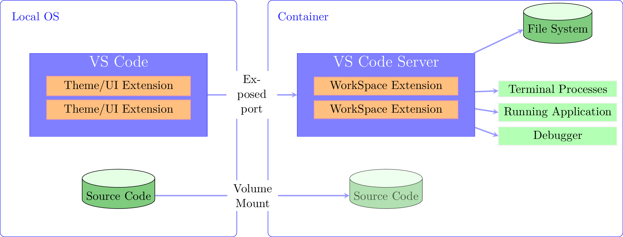
\end{tikzpicture}

\end{document} The code is a LaTeX document that generates a visualization of a development environment in the context of Visual Studio Code’s Remote Development feature. The visualization is a diagram created using the TikZ package, which shows the different components and their relationships within the development environment.

The diagram consists of two main elements: a “Local OS” box on the left-hand side, and a “Container” box on the right-hand side. The “Local OS” box represents the user’s computer, and the “Container” box represents a remote container that the user can connect to via Visual Studio Code’s Remote Development feature.

The diagram shows that Visual Studio Code is running on the user’s computer (“Local OS”), and that it is connected to a “VS Code Server” running in the remote container. The “VS Code Server” provides access to the user’s code and to the extensions and plugins that the user has installed.

The diagram also shows that the user’s code is stored in two “Source Code” databases: one on the user’s computer and one in the remote container. Other components in the diagram include “Theme/UI Extensions” and “Workspace Extensions” that are installed in Visual Studio Code, as well as “Terminal Processes,” “Running Application,” “Debugger,” and “File System” components that are part of the remote container. Arrows and labels are used to show the connections and relationships between the different components.

Block ] TikZ is a powerful and flexible tool for creating control systems diagrams, offering several benefits:

Customization: TikZ allows you to customize every aspect of your control systems diagrams, including the shapes, colors, fonts, and line styles. This level of customization makes it easy to create diagrams that fit your specific needs.
Integration: TikZ integrates seamlessly with LaTeX, allowing you to include your diagrams directly in your LaTeX documents. This integration ensures that your diagrams have the same font and formatting as the rest of your document.
Consistency: TikZ makes it easy to maintain consistency in your control systems diagrams, ensuring that all of your diagrams have the same look and feel. This consistency can make your diagrams easier to read and understand.
Flexibility: TikZ is a versatile tool that can be used to create a wide range of control systems diagrams, including block diagrams, signal flow graphs, and feedback control systems diagrams. This flexibility means that you can use TikZ for all of your control systems diagramming needs.
Collaboration: TikZ is an open-source tool that is widely used in the academic and scientific community. This popularity makes it easy to collaborate with others on control systems diagramming projects, as many people are familiar with TikZ and can easily contribute to your project.

Overall, TikZ is an excellent tool for creating control systems diagrams, offering customization, integration, consistency, flexibility, and collaboration benefits.

Using diagrams in documents

There are several ways to incorporate diagrams into LaTeX documents. Here are some of the most common methods:

TikZ: Use the TikZ package to create diagrams directly in your LaTeX document. TikZ offers a wide range of features and customization options, making it a powerful tool for creating diagrams.
External files: Create your diagrams in an external program, such as Inkscape or Adobe Illustrator, and save them as PDF files. Then, use the \includegraphics command to include the PDF files in your LaTeX document.
PGFPlots: Use the PGFPlots package to create advanced graphs and plots directly in your LaTeX document. PGFPlots offers a wide range of features for creating 2D and 3D plots, histograms, and more.
Circuitikz: Use the Circuitikz package to create circuit diagrams directly in your LaTeX document. Circuitikz offers a wide range of features for creating circuits with different components and styles.

Regardless of the method you choose, it is important to ensure that your diagrams are properly sized and aligned with the rest of your text. You may need to adjust the size of your diagrams or use LaTeX commands to properly align them with your text.

In summary, there are several methods for incorporating diagrams into LaTeX documents, including TikZ, external files, PGFPlots, and Circuitikz. Choose the method that best fits your needs and ensure that your diagrams are properly sized and aligned with the rest of your text.

When presenting diagrams in a professional manner, it is important to use figures and captions to help the reader understand the context and purpose of the diagram. Here is an overview of how to use figures and captions in LaTeX:

Use the \begin{figure} and \end{figure} commands to create a floating figure environment. This will allow LaTeX to place the diagram in the most suitable location, such as at the top or bottom of a page.
Use the \includegraphics command to insert the diagram into the figure environment. Be sure to specify the correct file path and size for the diagram.
Use the \caption command to provide a descriptive caption for the diagram. The caption should be brief, yet informative, and should explain the purpose of the diagram and any important features or results.
Use the \label command to label the figure with a unique identifier. This label can be used to refer to the figure in the text using the \ref command, which will automatically generate the correct figure number.
Place the figure and caption close to where it is first mentioned in the text. This will help the reader understand the context and purpose of the diagram.

In summary, using figures and captions can help to present diagrams in a professional manner by providing context and explanation for the reader. To use figures and captions in LaTeX, use the figure environment, insert the diagram with \includegraphics, provide a descriptive caption with \caption, label the figure with \label, and place the figure and caption close to where it is first mentioned in the text.

In LaTeX, it is common to refer to diagrams, figures, and other elements within the text of a document. Cross-referencing commands allow you to do this in a way that is consistent and efficient.

Here is an introduction to using cross-referencing commands to refer to diagrams in text:

Label the diagram with a unique identifier using the \label command. For example, you might label a diagram of a control system as \label{fig:controlsystem}.
Refer to the diagram in the text using the \ref command. For example, you might say “As shown in Figure \ref{fig:controlsystem}, the control system is composed of several feedback loops.”
Use the \autoref command to automatically generate a reference to the diagram with the appropriate label. For example, you might say “The control system is composed of several feedback loops (\autoref{fig:controlsystem}).”
Use the \nameref command to reference the name of the diagram. For example, you might say “For a detailed explanation of the control system, see \nameref{fig:controlsystem}.”

By using these cross-referencing commands, you can refer to diagrams in a way that is consistent and efficient, without having to manually update figure numbers or references if the position of the diagram changes within the document.

When working on technical documents, it is often necessary to include multiple diagrams or figures in a single section or chapter. LaTeX provides several packages that make it easy to place multiple diagrams in a single figure. Two such packages are subfig and wrapfig.

The subfig package allows you to create subfigures within a larger figure. Here is a brief overview of how to use subfig:

Load the subfig package by adding the following line to your document’s preamble: \usepackage{subfig}.
Create a figure that contains multiple subfigures using the \subfloat command. Here is an example:

\begin{figure}
 \centering
 \subfloat[Diagram A]{\includegraphics[width=0.4\textwidth]{diagramA}}
 \qquad
 \subfloat[Diagram B]{\includegraphics[width=0.4\textwidth]{diagramB}}
 \caption{Two diagrams.}
\end{figure}

In this example, two subfigures are created using the \subfloat command. The optional argument to \subfloat is a caption for each subfigure, and the mandatory argument is the image to be included.

Use the \caption command to provide a caption for the entire figure.

The wrapfig package allows you to place figures within the text flow, rather than in separate floating environments. Here is a brief overview of how to use wrapfig:

Load the wrapfig package by adding the following line to your document’s preamble: \usepackage{wrapfig}.
Use the \begin{wrapfigure} command to create a figure that is wrapped by text. Here is an example:

\begin{wrapfigure}{r}{0.5\textwidth}
 \centering
 \includegraphics[width=0.48\textwidth]{diagramC}
 \caption{Diagram C.}
\end{wrapfigure}

In this example, the optional argument to \begin{wrapfigure} specifies the placement of the figure (in this case, r for right). The mandatory argument is the width of the figure. The \includegraphics command is used to include the image, and the \caption command provides a caption for the figure.

By using packages such as subfig and wrapfig, you can create professional-looking documents with multiple diagrams in a single figure.

Getting started with tikz