Computing CAGR, volatility, Sharpe ratio and max drawdown in Python
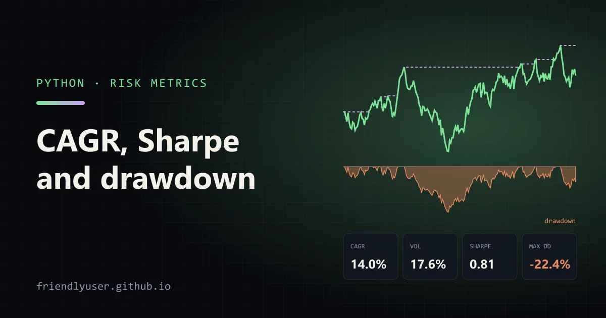
Four numbers show up on nearly every fund factsheet and backtest report: compound annual growth rate (CAGR), annualised volatility, the Sharpe ratio and maximum drawdown. Each one is a few lines of pandas, and each one has a common way to get it subtly wrong, usually in how daily numbers are turned into annual ones.
This post writes all four as small functions that take a daily price series, runs them on a reproducible synthetic series, and then shows the mistakes side by side with the correct numbers. Examples were run with Python 3.12, pandas and NumPy.
Simple and log returns
Section titled “Simple and log returns”Everything starts from daily returns, and there are two kinds:
- Simple return:
p[t] / p[t-1] - 1. This is what you earned. Simple returns of different assets on the same day add across a portfolio: a 50/50 portfolio’s return is the average of the two. - Log return:
ln(p[t] / p[t-1]). Log returns add across time: the sum of daily log returns is the log of the total return.
Neither is wrong; they answer different questions. Mixing them up causes most of the errors at the end of this post.
The metrics
Section titled “The metrics”Save this as metrics.py:
"""Return and risk metrics from a daily price series."""import numpy as npimport pandas as pd
TRADING_DAYS = 252

def cagr(prices: pd.Series) -> float:    years = (prices.index[-1] - prices.index[0]).days / 365.25    return (prices.iloc[-1] / prices.iloc[0]) ** (1 / years) - 1

def annual_volatility(prices: pd.Series) -> float:    daily = prices.pct_change().dropna()    return daily.std() * np.sqrt(TRADING_DAYS)

def sharpe_ratio(prices: pd.Series, risk_free_annual: float = 0.0) -> float:    daily = prices.pct_change().dropna()    rf_daily = (1 + risk_free_annual) ** (1 / TRADING_DAYS) - 1    excess = daily - rf_daily    return excess.mean() / excess.std() * np.sqrt(TRADING_DAYS)

def drawdown(prices: pd.Series) -> pd.Series:    """Fraction below the running peak, 0 at new highs."""    return prices / prices.cummax() - 1

def max_drawdown(prices: pd.Series) -> dict:    dd = drawdown(prices)    trough = dd.idxmin()    peak = prices.loc[:trough].idxmax()    after = prices.loc[trough:]    recovered = after[after >= prices.loc[peak]]    return {        "max_drawdown": dd.min(),        "peak": peak.date(),        "trough": trough.date(),        "recovered": recovered.index[0].date() if len(recovered) else None,    }

def synthetic_prices(seed: int = 5, years: int = 5) -> pd.Series:    rng = np.random.default_rng(seed)    n = years * TRADING_DAYS    log_ret = rng.normal(0.08 / TRADING_DAYS - 0.5 * 0.18**2 / TRADING_DAYS, 0.18 / np.sqrt(TRADING_DAYS), n)    index = pd.bdate_range("2021-01-04", periods=n)    return pd.Series(100 * np.exp(np.cumsum(log_ret)), index=index)

if __name__ == "__main__":    prices = synthetic_prices()    print(f"days:        {len(prices)}  ({prices.index[0].date()} to {prices.index[-1].date()})")    print(f"total:       {prices.iloc[-1] / prices.iloc[0] - 1:.2%}")    print(f"CAGR:        {cagr(prices):.2%}")    print(f"volatility:  {annual_volatility(prices):.2%}")    print(f"Sharpe (0%): {sharpe_ratio(prices):.2f}")    print(f"Sharpe (4%): {sharpe_ratio(prices, 0.04):.2f}")    for k, v in max_drawdown(prices).items():        print(f"{k + ':':<13}{v:.2%}" if isinstance(v, float) else f"{k + ':':<13}{v}")
CAGR is the constant yearly rate that turns the starting value into the ending value:
CAGR = (end / start) ** (1 / years) - 1
The only decision is how to count years. The function uses the calendar time between the first and last dates, which is correct whatever the data frequency and however many holidays the series has.
Volatility
Section titled “Volatility”Annualised volatility is the standard deviation of daily returns times the square root of the number of trading periods in a year. The square root comes from assuming daily returns are independent: variances add over time, so standard deviations grow with the square root. 252 is the usual count of trading days in a US year. Use 12 for monthly data, 52 for weekly, and 365 for assets that trade every day, such as crypto.
Sharpe ratio
Section titled “Sharpe ratio”The Sharpe ratio is the average return above the risk-free rate, divided by the volatility of that excess return. With daily data:
- Convert the annual risk-free rate to a daily one:
(1 + rf) ** (1/252) - 1. - Subtract it from each daily return.
- Divide the mean excess return by its standard deviation and multiply by
sqrt(252).
The risk-free rate should match the period and currency of the returns, typically a short-term Treasury bill yield for US dollar assets. A Sharpe ratio computed with 0% and one computed with 4% are not comparable, so always report which rate you used.
Drawdown
Section titled “Drawdown”The drawdown on each day is how far the price is below its highest value so far, prices / prices.cummax() - 1. Maximum drawdown is the minimum of that series. The max_drawdown function also returns the peak before the worst trough, the trough itself, and the first day the price got back to the old peak, if it did. Recovery time is often more informative than the depth.
Running it
Section titled “Running it”The synthetic series is five years of a seeded random walk with 8% drift and 18% volatility, so the numbers are reproducible but describe no real asset:
pip install pandas numpypython metrics.pydays: 1260 (2021-01-04 to 2025-10-31)total: 88.35%CAGR: 14.03%volatility: 17.55%Sharpe (0%): 0.81Sharpe (4%): 0.59max_drawdown:-22.43%peak: 2021-01-18trough: 2021-05-27recovered: 2022-09-15The worst drawdown started two weeks in, bottomed out four months later, and took until September 2022 to recover: 20 months under water for a series that ended up 88%.
To run on real prices, pass any pd.Series of daily closes with a DatetimeIndex, adjusted for dividends and splits.
The pitfalls, measured
Section titled “The pitfalls, measured”This script computes several plausible-looking alternatives on the same series:
import numpy as npfrom metrics import TRADING_DAYS, cagr, synthetic_prices
prices = synthetic_prices()simple = prices.pct_change().dropna()log = np.log(prices).diff().dropna()
print(f"CAGR:                        {cagr(prices):.2%}")print(f"mean simple return x 252:    {simple.mean() * TRADING_DAYS:.2%}")print(f"mean log return x 252:       {log.mean() * TRADING_DAYS:.2%}")print(f"exp(that) - 1:               {np.expm1(log.mean() * TRADING_DAYS):.2%}")print(f"sum of simple returns:       {simple.sum():.2%}")print(f"actual total return:         {prices.iloc[-1] / prices.iloc[0] - 1:.2%}")print(f"vol with sqrt(252):          {simple.std() * np.sqrt(252):.2%}")print(f"vol with sqrt(365):          {simple.std() * np.sqrt(365):.2%}")
CAGR: 14.03%mean simple return x 252: 14.21%mean log return x 252: 12.67%exp(that) - 1: 13.51%sum of simple returns: 71.01%actual total return: 88.35%vol with sqrt(252): 17.55%vol with sqrt(365): 21.13%What each line shows:
- Average simple return is not the growth rate. The arithmetic mean of daily returns, annualised, is above what you actually compounded at. The gap between it and the mean log return (14.21% vs 12.67%) is about half the variance,
0.1755² / 2 ≈ 1.5%. This is volatility drag: losing 10% and then gaining 10% leaves you below where you started. - Summing simple returns is wrong over time. 71% vs an actual 88%. Simple returns compound; only log returns add.
- The calendar and the trading-day count can disagree.
exp(mean log x 252) - 1should equal CAGR, but here it’s 13.51% vs 14.03%. The synthetic index usesbdate_range, which has every weekday and no holidays, about 261 days a year. Scaling by 252 then implies more years than the calendar shows. Real US equity data has roughly 252 sessions a year, so the two methods agree closely there. When they don’t, check your data’s frequency before trusting either. - The annualisation factor matters. Using
sqrt(365)on data that only has trading days inflates volatility by about 20%, becausesqrt(365/252) ≈ 1.20. Many crypto-versus-stock comparisons make this mistake in one direction or the other.
Other gotchas
Section titled “Other gotchas”- Use adjusted prices. Unadjusted closes drop on ex-dividend days and splits. A 4-for-1 split looks like a 75% drawdown.
- Missing days. If a series has gaps (a suspended stock, a data outage),
pct_changeproduces a multi-day return on the first day back, and volatility is understated. Don’t forward-fill a price and treat the flat days as zero-return trading days. - Sharpe assumes independent, roughly symmetric returns. Strategies that sell options or hold illiquid assets can show a high Sharpe until a rare large loss. Look at the drawdown and the worst days as well.
- Short histories. A Sharpe ratio from one or two years of data has a wide margin of error. A difference between 0.6 and 0.8 over two years is not meaningful.
- Portfolios. For a portfolio, compute daily portfolio values (or the weighted sum of simple returns) first, then apply these functions. Don’t average the assets’ CAGRs or Sharpe ratios.
Further reading
Section titled “Further reading”© 2026 David Li · Home · Blog · RSS ·Classic site · Built with Astro, Starlight and three.js · Logos:Font Awesome Free (CC BY 4.0)