Backtesting a moving-average crossover in pandas without look-ahead bias
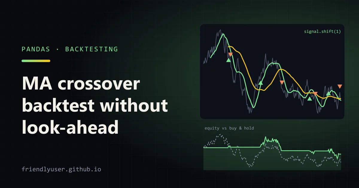
A moving-average crossover is the “hello world” of trading strategies: hold the asset while a fast average of the price is above a slow one, and stay in cash otherwise. It is simple enough to backtest in a dozen lines of pandas, which is exactly why it is a good way to learn the mistakes that make backtests lie.
This post builds that backtest step by step, with the signal computed on the close and the trade taken on the next bar, transaction costs, and a comparison against buy and hold. All the numbers come from synthetic prices, a seeded random walk, so you can reproduce them exactly. The code was run with Python 3.12, pandas and NumPy.
The data
Section titled “The data”Random-walk prices have one useful property for this exercise: by construction, there is no trend signal in them for a crossover to find. Any profit a strategy shows on them is luck or a bug.
import numpy as npimport pandas as pd
TRADING_DAYS = 252

def synthetic_prices(seed: int, years: int = 10, drift: float = 0.07, vol: float = 0.20) -> pd.Series:    """Geometric Brownian motion: a random walk with no exploitable trend signal."""    rng = np.random.default_rng(seed)    n = years * TRADING_DAYS    daily = rng.normal(drift / TRADING_DAYS - 0.5 * vol**2 / TRADING_DAYS, vol / np.sqrt(TRADING_DAYS), n)    dates = pd.bdate_range("2016-01-04", periods=n)    return pd.Series(100 * np.exp(np.cumsum(daily)), index=dates, name="close")
To use real data instead, any daily close series with a DatetimeIndex works. With the yfinance package, for example (prices adjusted for splits and dividends):
import yfinance as yf
close = yf.download("SPY", start="2010-01-01", end="2025-12-31",                    auto_adjust=True, progress=False)["Close"]["SPY"]
yf.download returns a frame with a column level per ticker, hence the ["SPY"] to get a plain Series. Use adjusted prices; raw closes drop on every dividend and split, and a backtest reads those drops as losses.
The backtest
Section titled “The backtest”Append this to backtest.py:
def backtest(close: pd.Series, fast: int = 50, slow: int = 200, cost_bps: float = 10, lag: int = 1) -> pd.DataFrame:    df = pd.DataFrame({"close": close})    df["fast"] = df["close"].rolling(fast).mean()    df["slow"] = df["close"].rolling(slow).mean()    # Signal is known at the close of day t ...    df["signal"] = (df["fast"] > df["slow"]).astype(int)    # ... so the earliest it can earn a return is day t+1.    df["position"] = df["signal"].shift(lag).fillna(0)    df["ret"] = df["close"].pct_change().fillna(0)    df["trades"] = df["position"].diff().abs().fillna(0)    df["strategy_ret"] = df["position"] * df["ret"] - df["trades"] * cost_bps / 10_000    df = df.iloc[slow:]                      # drop the warm-up period    df["strategy"] = (1 + df["strategy_ret"]).cumprod()    df["buy_hold"] = (1 + df["ret"]).cumprod()    return df

def summary(equity: pd.Series) -> dict:    years = len(equity) / TRADING_DAYS    cagr = equity.iloc[-1] ** (1 / years) - 1    max_dd = (equity / equity.cummax() - 1).min()    return {"total": f"{equity.iloc[-1] - 1:.1%}", "cagr": f"{cagr:.1%}", "max_dd": f"{max_dd:.1%}"}

if __name__ == "__main__":    close = synthetic_prices(seed=7)    honest = backtest(close)    cheating = backtest(close, lag=0)    print("buy & hold     ", summary(honest["buy_hold"]))    print("crossover      ", summary(honest["strategy"]), "trades:", int(honest["trades"].sum()))    print("look-ahead bug ", summary(cheating["strategy"]))
Line by line, the parts that matter:
rolling(...).mean()only uses the current and past values, so the averages themselves don’t peek ahead.rolling(window, center=True)would, and so would any smoothing fitted on the whole series.signalis 1 when the fast average is above the slow one, decided from day t’s close.position = signal.shift(1)is the line that prevents look-ahead bias.reton day t is the close-to-close return from t-1 to t. If you multiply it by the signal from the same day, you are using day t’s close to decide whether to own the stock during the move that produced that close. Shifting by one bar means the return on day t is earned by a decision made at t-1.tradesis 1 on each day the position changes. Each change costscost_bpsbasis points (10 bps = 0.1%), a rough stand-in for commission, bid-ask spread and slippage.iloc[slow:]drops the first 200 days, where the slow average doesn’t exist yet. Both curves start on the same day, so the comparison is fair.
Results on one series
Section titled “Results on one series”python backtest.pybuy & hold {'total': '-22.5%', 'cagr': '-2.7%', 'max_dd': '-55.5%'}crossover {'total': '-11.8%', 'cagr': '-1.4%', 'max_dd': '-31.9%'} trades: 21look-ahead bug {'total': '-1.4%', 'cagr': '-0.2%', 'max_dd': '-25.0%'}On this seed, the random walk drifted down, and the crossover lost less than buy and hold, with a much smaller drawdown. It is tempting to read that as “trend following protects you in bear markets”. Remember there is no trend signal in this data to follow.
The third line is the same strategy without the shift (lag=0). The only difference is a one-day timing error, and it adds about ten percentage points of total return. With slower signals like a 200-day average, look-ahead bias is modest. With daily signals that flip often, it can turn a losing strategy into a spectacular one, which is why a backtest that looks too good is usually a bug.
To see the equity curves:
import matplotlib.pyplot as pltfrom backtest import backtest, synthetic_prices
bt = backtest(synthetic_prices(seed=7))ax = bt[["strategy", "buy_hold"]].plot(figsize=(9, 4), title="Growth of 1 (synthetic data, seed 7)")ax.set_ylabel("equity")plt.tight_layout()plt.savefig("equity.png", dpi=120)
Why one series proves nothing
Section titled “Why one series proves nothing”Run the same backtest on 200 random walks, all with the same drift and volatility, and compare each strategy’s CAGR with buy and hold on the same path:
import pandas as pd
from backtest import TRADING_DAYS, backtest, synthetic_prices

def cagr(equity: pd.Series) -> float:    return equity.iloc[-1] ** (TRADING_DAYS / len(equity)) - 1

rows = []for seed in range(200):    bt = backtest(synthetic_prices(seed))    rows.append({"seed": seed, "excess_cagr": cagr(bt["strategy"]) - cagr(bt["buy_hold"])})
excess = pd.DataFrame(rows)["excess_cagr"]print(f"crossover beat buy & hold on {(excess > 0).sum()} of {len(excess)} random walks")print(f"best seed:  {excess.max():+.1%} a year")print(f"worst seed: {excess.min():+.1%} a year")print(f"median:     {excess.median():+.1%} a year")
crossover beat buy & hold on 59 of 200 random walksbest seed: +8.4% a yearworst seed: -12.2% a yearmedian: -2.4% a yearOn data with no signal at all, the crossover beat buy and hold on 59 paths, one of them by 8.4% a year over about nine years. If that path were a real ticker you had picked, the backtest would look like a discovery. The median result is negative because, on an upward-drifting random walk, sitting in cash part of the time misses some of the drift and pays costs on every switch.
That is the core problem with testing one strategy on one ticker: the spread of outcomes from luck alone is wide, and a single backtest is one draw from it. Before trusting a result, at minimum:
- test across many assets and time periods, not the one where you noticed the pattern;
- hold out data you never looked at while choosing
fastandslow; - count how many parameter combinations you tried, because the best of fifty is biased upward even if each test is honest.
Gotchas
Section titled “Gotchas”- Survivorship bias. Today’s index members are the companies that survived. Backtesting them over the past ten years leaves out the ones that went bankrupt or were delisted.
- Fills.
shift(1)assumes you trade at the close the signal came from, which requires a market-on-close order placed with a signal computed just before the close. Trylag=2to see how sensitive the result is to a one-day delay. If it collapses, the edge was timing, not trend. - Costs are not constant. 10 bps is plausible for a liquid ETF and far too low for small caps or for size that moves the price.
- Cash earns interest. This backtest earns zero when out of the market. Over a period with meaningful interest rates, that understates the strategy; add a daily risk-free return on days with
position == 0if it matters. - Taxes. Every exit in a taxable account can realise a gain. Buy and hold defers that; frequent switching does not.
- Event-driven frameworks. A vectorised backtest like this one is fast and transparent, but it gets awkward for stops, position sizing or multiple assets. At that point a library such as backtrader or vectorbt handles the bookkeeping.
Further reading
Section titled “Further reading”© 2026 David Li · Home · Blog · RSS ·Classic site · Built with Astro, Starlight and three.js · Logos:Font Awesome Free (CC BY 4.0)