How Parquet files work: row groups, column chunks and statistics
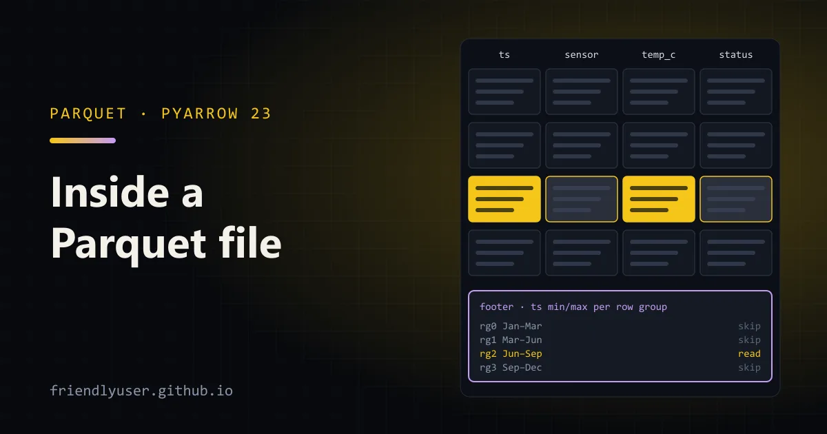
Parquet is a columnar file format for tabular data. Instead of storing one row after another like CSV, it stores each column’s values together, compressed, with enough metadata that a reader can skip the columns and the chunks of rows a query doesn’t need. That’s why the same data is usually several times smaller as Parquet than as CSV, and why DuckDB, Polars, Spark and pandas can query it so quickly.
You can use Parquet without knowing its layout, but a few minutes with the structure explains most of its performance tips. This post looks inside a real file with pyarrow.parquet. Examples use PyArrow 23.0 on Python 3.13.
The layout
Section titled “The layout”A Parquet file is organized in three levels:
readings.parquet├── "PAR1" magic bytes├── Row group 0 (rows 0 .. 249,999)│ ├── Column chunk: ts ─┐│ ├── Column chunk: sensor │ each chunk = an optional dictionary page│ ├── Column chunk: temp_c │ + data pages, compressed│ └── Column chunk: status ─┘├── Row group 1 (rows 250,000 .. 499,999)│ └── ...├── ...├── Footer (FileMetaData) schema, row group list, per-chunk offsets,│ encodings, sizes and min/max statistics├── footer length (4 bytes)└── "PAR1"- A row group is a horizontal slice of the table: a batch of rows.
- Inside each row group, every column is stored as a column chunk: all of that column’s values for those rows, contiguous on disk.
- Each chunk is split into pages, the unit of encoding and compression.
- The footer at the end describes everything. A reader seeks to the end, reads the footer length, reads the footer, and from then on knows the byte offset of every column chunk.
Because the metadata is at the end, a writer can stream rows out and write the footer last. And because the footer has offsets, a reader that wants two columns from one row group reads exactly those byte ranges. Over HTTP or S3, that’s a handful of range requests rather than the whole file.
Writing a file to inspect
Section titled “Writing a file to inspect”This creates a million sensor readings, sorted by time, and writes them with four row groups:
import datetime as dtimport random
import pyarrow as paimport pyarrow.parquet as pq
random.seed(7)n = 1_000_000start = dt.datetime(2026, 1, 1)table = pa.table({    "ts": pa.array([start + dt.timedelta(seconds=30 * i) for i in range(n)], pa.timestamp("ms")),    "sensor": pa.array([f"s{random.randrange(50):02d}" for _ in range(n)]),    "temp_c": pa.array([round(random.gauss(21, 3), 2) for _ in range(n)], pa.float64()),    "status": pa.array(random.choices(["ok", "ok", "ok", "warn", "fail"], k=n)),})
pq.write_table(table, "readings.parquet", row_group_size=250_000, compression="zstd")
row_group_size is a maximum number of rows. If you leave it out, PyArrow caps row groups at 1,048,576 rows (1024 × 1024); a 2.5-million-row table came out as groups of 1,048,576, 1,048,576 and 402,848.
You can check the magic bytes yourself:
import struct
data = open("readings.parquet", "rb").read()print(data[:4], data[-4:], struct.unpack("<i", data[-8:-4])[0])# b'PAR1' b'PAR1' 2288     <- the footer is 2,288 bytes
Reading the footer with pyarrow.parquet
Section titled “Reading the footer with pyarrow.parquet”pq.ParquetFile reads only the footer when you open it, so this is fast even on huge files:
import pyarrow.parquet as pq
pf = pq.ParquetFile("readings.parquet")md = pf.metadataprint(md)
<pyarrow._parquet.FileMetaData object at 0x...> created_by: parquet-cpp-arrow version 23.0.1 num_columns: 4 num_rows: 1000000 num_row_groups: 4 format_version: 2.6 serialized_size: 2288pq.read_metadata(path) and pq.read_schema(path) are shortcuts when you only need those. Drill into a row group and a column chunk:
print(md.row_group(0).column(2)) # temp_c in row group 0<pyarrow._parquet.ColumnChunkMetaData object at 0x...> file_offset: 0 file_path: physical_type: DOUBLE num_values: 250000 path_in_schema: temp_c is_stats_set: True statistics: <pyarrow._parquet.Statistics object at 0x...> has_min_max: True min: 8.17 max: 34.98 null_count: 0 distinct_count: None num_values: 250000 physical_type: DOUBLE logical_type: None converted_type (legacy): NONE geo_statistics: None compression: ZSTD encodings: ('PLAIN', 'RLE', 'RLE_DICTIONARY') has_dictionary_page: True dictionary_page_offset: 1280280 data_page_offset: 1286402 total_compressed_size: 359233 total_uncompressed_size: 376144Each column chunk knows its byte offset, its encodings, its compressed and uncompressed size, and its statistics: min, max and null count.
Statistics and predicate pushdown
Section titled “Statistics and predicate pushdown”Those min/max values are what make filters cheap. Here are the ts statistics for each row group:
for i in range(md.num_row_groups): rg = md.row_group(i) st = rg.column(0).statistics print(i, rg.num_rows, st.min, st.max)0 250000 2026-01-01 00:00:00 2026-03-28 19:19:301 250000 2026-03-28 19:20:00 2026-06-23 14:39:302 250000 2026-06-23 14:40:00 2026-09-18 09:59:303 250000 2026-09-18 10:00:00 2026-12-14 05:19:30A query for the first week of July can only match row group 2, because every other group’s ts range excludes it. Readers check the statistics first and skip the rest without decompressing them. That’s predicate pushdown. Combined with reading only the needed columns (projection pushdown), a query may touch a small fraction of the file.
With PyArrow, pass filters and columns:
import datetime as dt
t = pq.read_table(    "readings.parquet",    columns=["ts", "temp_c"],    filters=[("ts", ">=", dt.datetime(2026, 7, 1)), ("ts", "<", dt.datetime(2026, 7, 8))],)print(t.num_rows)   # 20160
You can see which row groups survive the filter with the dataset API:
import pyarrow as paimport pyarrow.compute as pcimport pyarrow.dataset as ds
flt = (pc.field("ts") >= pa.scalar(dt.datetime(2026, 7, 1), pa.timestamp("ms"))) & (    pc.field("ts") < pa.scalar(dt.datetime(2026, 7, 8), pa.timestamp("ms")))frag = next(ds.dataset("readings.parquet", format="parquet").get_fragments())print(frag.num_row_groups, [f.row_groups[0].id for f in frag.split_by_row_group(flt)])# 4 [2]
The catch: statistics only help if values are clustered. The ts ranges are tight because the data was written in time order. If the rows were shuffled, every row group would span the whole year and nothing could be skipped. sensor is random in this file, so a filter on sensor == "s07" can’t skip any row group. If you filter on a column often, sort by it before writing.
PyArrow can also write a page index (write_page_index=True), which stores min/max per page as well as per chunk, so readers that support it can skip at a finer grain.
Compression codecs
Section titled “Compression codecs”Compression is applied per page, after encoding. Writing the same table with each codec:
import os
for codec in ["none", "snappy", "lz4", "gzip", "zstd"]:    path = f"c_{codec}.parquet"    pq.write_table(table, path, row_group_size=250_000, compression=codec)    print(f"{codec:7} {os.path.getsize(path) / 1e6:6.2f} MB")
none 11.60 MBsnappy 9.03 MBlz4 9.04 MBgzip 6.18 MBzstd 6.74 MBThat’s one synthetic dataset; your ratios will differ. In general, Snappy (PyArrow’s default) and LZ4 are fast with modest compression, gzip compresses well but is slow to decompress, and Zstandard gets close to gzip’s size while decompressing much faster. You can tune it with compression_level. Zstd is a good default for files that are written once and read many times.
Encodings matter as much as codecs
Section titled “Encodings matter as much as codecs”Before compression, values are encoded. By default PyArrow tries dictionary encoding for every column: it stores each distinct value once and replaces the values with small integer indexes, falling back to plain encoding when the dictionary gets too big. That’s ideal for sensor (50 distinct values) and status (3), and it’s why repetitive string columns compress so well in Parquet.
It’s poor for the ts column, where every value is distinct. In the file above, each ts chunk was about 1.09 MB. Timestamps sorted at a fixed interval are a perfect fit for delta encoding, which stores the differences between consecutive values:
pq.write_table( table, "delta.parquet", row_group_size=250_000, compression="zstd", use_dictionary=["sensor", "status"], # dictionary only where it helps column_encoding={"ts": "DELTA_BINARY_PACKED"},)md = pq.ParquetFile("delta.parquet").metadataprint(md.row_group(0).column(0).total_compressed_size) # 1429The ts chunk shrank from about 1.09 MB to 1,429 bytes, and the whole file from 6.74 MB to 3.58 MB. Real timestamps aren’t perfectly regular, so expect less, but sorted integer and timestamp columns usually benefit. column_encoding requires turning dictionary encoding off for those columns, which is why use_dictionary lists only the string columns.
Partitioned datasets
Section titled “Partitioned datasets”For data that keeps growing, a single file isn’t practical. The common layout is a directory of Parquet files partitioned by one or more columns, Hive style:
import pyarrow.compute as pcimport pyarrow.dataset as ds
with_parts = ( table.append_column("year", pc.year(table["ts"])) .append_column("month", pc.month(table["ts"])))ds.write_dataset( with_parts, "readings_by_month", format="parquet", partitioning=["year", "month"], partitioning_flavor="hive", existing_data_behavior="overwrite_or_ignore",)readings_by_month/year=2026/month=1/part-0.parquetreadings_by_month/year=2026/month=2/part-0.parquet...readings_by_month/year=2026/month=12/part-0.parquetThe partition columns live in the directory names, not inside the files. Readers that understand Hive partitioning add them back as columns, and a filter on them skips whole files before opening anything:
part = ds.dataset("readings_by_month", format="parquet", partitioning="hive")flt = (pc.field("month") == 7) & (pc.field("status") == "fail")print(len(list(part.get_fragments(filter=flt)))) # 1 file to readprint(part.to_table(filter=flt, columns=["sensor", "temp_c"]).num_rows) # 17858The same directory works with pl.scan_parquet("readings_by_month/**/*.parquet", hive_partitioning=True) in Polars and read_parquet(..., hive_partitioning = true) in DuckDB.
Partition on columns you filter by and that have a modest number of values (dates, regions). Partitioning on something with thousands of values produces thousands of tiny files, and the per-file overhead then costs more than the skipping saves.
Gotchas and rules of thumb
Section titled “Gotchas and rules of thumb”- Small files are slow. Every file and row group has fixed overhead. Aim for row groups of tens to hundreds of MB and avoid writing one file per small batch; compact them later if you must.
- Sort before writing by the columns you filter on, so statistics can skip row groups.
- Parquet files are immutable. You can’t update a row in place. Table formats like Delta Lake and Apache Iceberg add transactions, deletes and schema evolution on top of directories of Parquet files.
- Schemas must line up across files in a dataset. A column that is
int64in one file anddoublein another causes errors or surprise casts; pass an explicitschematods.datasetif the files drifted. - Timestamps and time zones. Store UTC with a time zone (
pa.timestamp("ms", tz="UTC")) if the meaning matters; naive timestamps are read back as naive.
Further reading
Section titled “Further reading”- Apache Parquet documentation, including the file format and encodings pages
- Reading and writing Parquet with PyArrow
- Tabular datasets in PyArrow
© 2026 David Li · Home · Blog · RSS ·Classic site · Built with Astro, Starlight and three.js · Logos:Font Awesome Free (CC BY 4.0)